5.3 Running the script for automatic photometry

The AsPyLib script for automatic photometry has been used with a series of images of a star field in Cassiopeia. The images have been taken on 14 November 2011. Several variable stars have been found, some of them are already known, others are unknown. We show here the various step of the variable star detection.

464 images have been taken during a period of 4h45. A ST8300 camera, in binning 2x2 has been used (1676*1266 pixels). The field of view is about 0.8 deg*0.6 deg.

Star detection

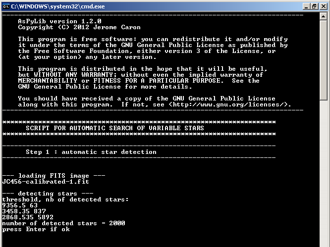
The first step that is performed by the script is the star detection. In the script text, we specified:

nbtarget = 2000

The script thus selects the 2000 brightest stars. The saturated stars are disregarded because they will give inaccurate photometry:

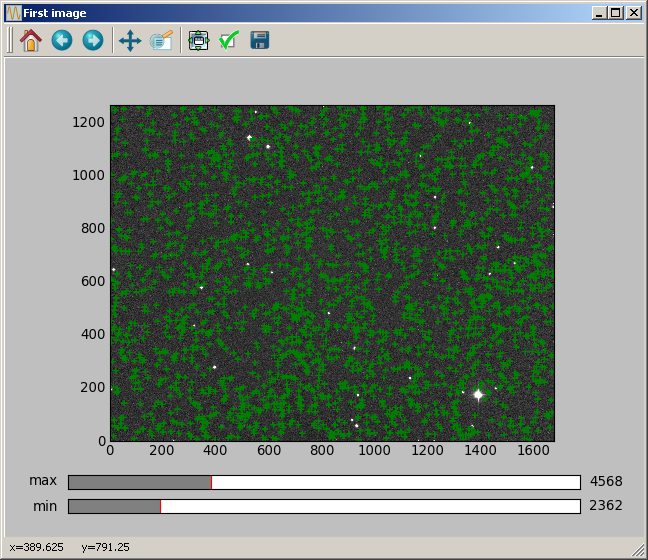
We can zoom in to see better the detected stars:

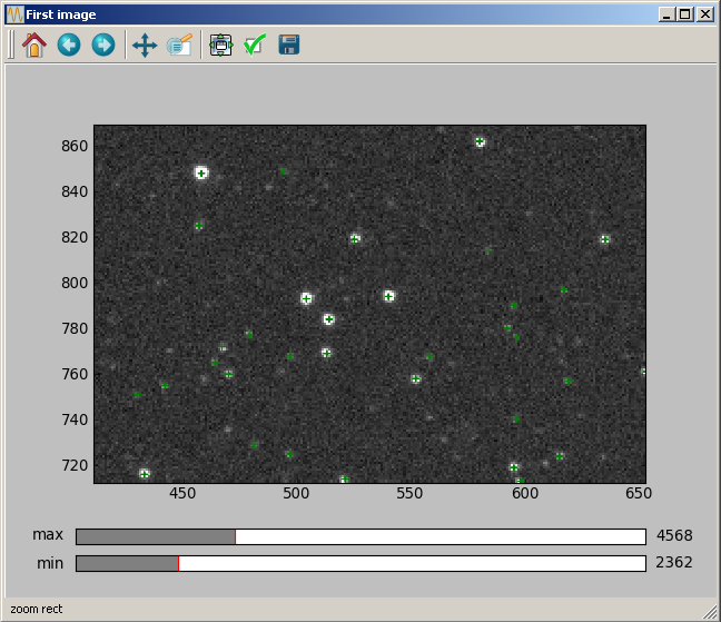
Everything is ok, so we press “Enter”:

Checking input images

The next step is a carefull check of all input images. First, the dynamic range (as the difference between the max and min values in a certain area of the picture) is computed. The user must decide whether the min and max are calculated over the complete image (option 1) or on a subpart of the image (option 2).

We choose option 2 (typing: 2 + Enter) to define a small rectangle which will not contain any saturated star. We select 4 points with mouse right-clicks, approximately corresponding to the corners of the rectangle in red below. The script calculates the smallest rectangle that encloses the 4 selected positions. This rectangle will be used to compute the min signal, max signal and dynamic range:

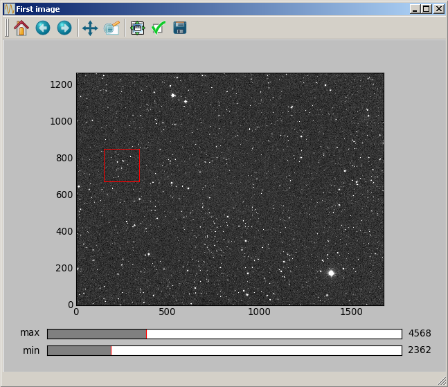
All pictures are loaded, and after a short time the following curve appears.

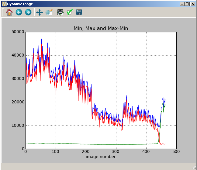
The green curve gives the minimum signal (in that case, close to 0), the blue curve gives the maximum and the red one the difference max-min.

At the end of the night, we see that the signal is strongly decreasing (red curve) and the background increases (green curve). This happens because the observed star field disappears behind a tree. The user has the option to remove images with too low signal:

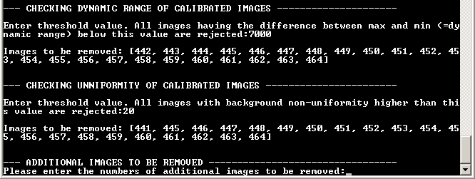
We choose a threshold at 7000 (typing: 7000 + Enter).

A new figure then appears, that represents the background uniformity. Background uniformity is calculated as the difference between median values in different areas of the image. The curves show that the uniformity is acceptable except at the end of the night where strong heterogeneities appear. This decrease of image homogeneity is a quite reliable signature of obstacles like trees, roof, etc (much more reliable than changes in the signal strength).

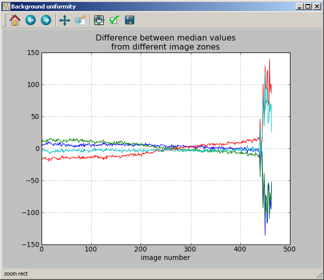
The user has the possibility to remove images by specifying a threhold. We choose a threshold at 20 (typing: 20 + Enter).

Next we have the possibility to reject additional pictures. This can be useful if, for instance, we know that one image in the middle of the night went wrong, due to some bright satellite passing, or to mount vibration, etc. We choose not to reject any image, so we just press “Enter”. Finally, the complete list of rejected images appears:

Computing image shifts

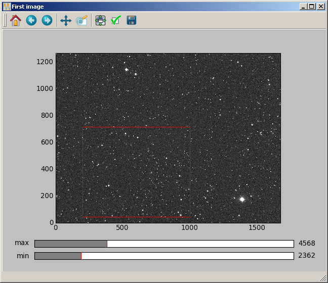
The next step is to calculate the shifts of all images in the series with respect to the first image. To do it, we have 3 possibilities. Stars can be detected over the full image (option 1), over the full image except some parts of it (option 2), or over a subpart of the image (option 3).

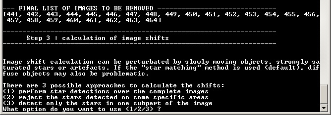
Since we have one star that is strongly saturated, we choose option 3 (typing: 3 + Enter). We are asked to select with the mouse a rectangle in the picture. We do it by right-clicking approximately on the 4 corners of the rectangle in red below.

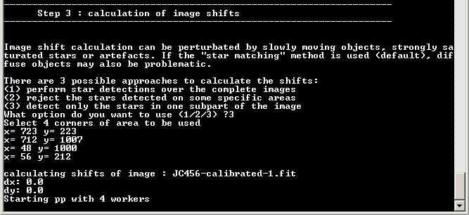
Next, the script calculates the image shifts in the series. Parallel processing is used (here with 4 processors) to speed up calculations. The calculation of image shifts is done separately from the photometry, in order to visualise the complete curve of the (X,Y) shifts and to see immediately if some image shift was wrongly calculated. Then the user can reject these images before a wrong photometry is calculated. After a short time, the plot of the X and Y shifts appears:

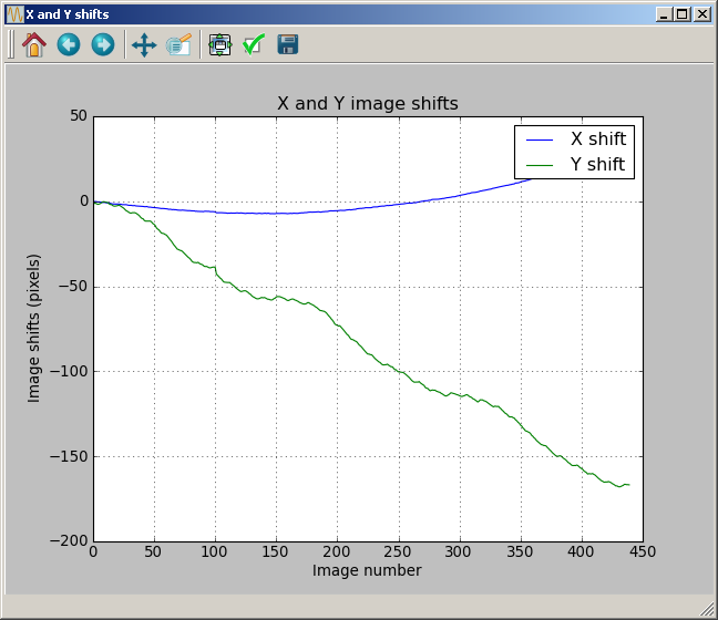
It is very nice to see the effect of incorrect polar pointing of the mount (average drift of each curve) and the periodic errors of the mount in the alpha axis (Y shift). We now have the possibility to reject some images.

Since the calculation was correct, we just type “Enter”.

Photometry calculations and processing

Next, the aperture photometry calculation start (still in parallel processing):

After a short time, the photometry is completed.

The script removes the stars that have more than 20% of their measurement incorrect (e.g. star outside image, saturated star or negative intensity).

Then it identifies the stars having 100% of correct measurements. They are considered as candidates for being reference stars. From the 40 brightest stars in this set, the script selects the best combination of 20 reference stars. Then it calculates differential magnitudes and statistics.

Final results

Finally the script exports all results to a text file (here “JC456_03_magnitudes.txt”).

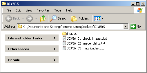
The text file with the magnitudes data contains the following information:

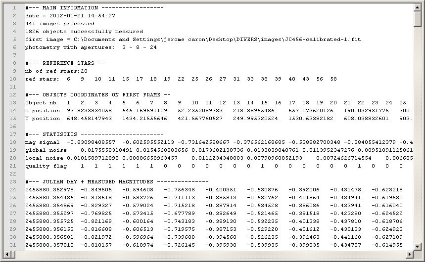
In particular, for each object the average magnitude, the “global noise” and “local noise” are computed (see here for explanations). A quality flag is also calculated, equal to:

• -1 if more than 20% of the measurements were wrong and the star was removed
• otherwise, a number between 0 and 4 giving the quality of the lightcurve (0 for the best quality, 4 for the worse quality)

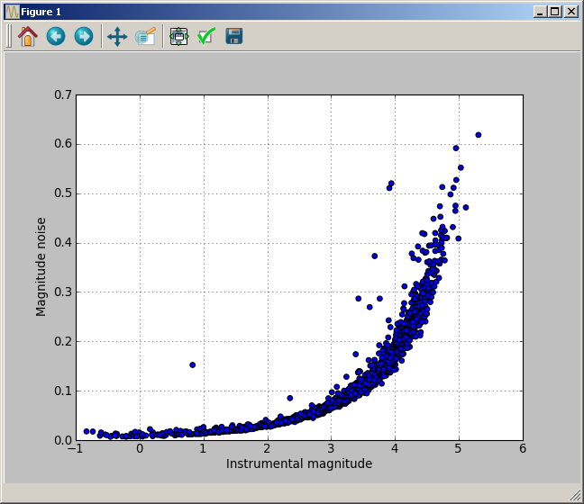
To conclude the script execution, a simple plot showing the magnitude noise (“global noise”) as a function of magnitude is shown. This plot gives a good idea of the smallest noise values achieved, the faintest stars measured, and the quantity of false detections.