5.4 Search for variable stars in the measured data

Once the magnitudes of all stars have been calculated and exported in a text file, all the information is there but only half of the job been made. The remaining part is to find which stars are variable.

For this, one can use the script “05_photometry\photosearch_viewresults.py”.

Input parameters

To run the script, 3 input parameters are required.

The first one is the name of the file that was generated by the script for automatic photometry, which contains all the magnitude data:

File = "C:\\processing\\target_03_magnitudes.txt"

Once again, it is possible to write some extra code here, for instance to separate the folder and file names:

Folder = u"C:\\processing\\"
File = Folder + 'target_' + "03_magnitudes.txt"

The second parameter is the number of stars the user wants to display at once. We recommend to keep it equal to 1, but one can also change it to see what happens...

nb_stars = 1

Finally, the ‘mode’ parameter defines whether the complete set of data will be displayed in a “global noise” vs magnitude plot, or in a “local noise” vs “global noise” plot. Both approaches work fine, so it’s mostly a matter of preference.

mode = 1

#mode = 1 --> plot is magnitude / global noise
#mode = 2 --> plot is local noise / global noise

Running the script

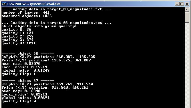
When running the script, at first some information is displayed in the console window, and a figure appears.

In the console, the number of images and the number of objects successfully measured (i.e. the ones with more than 80% of measurements being successful) are shown. In our case, 174 objects could not be measured. The majority of them are stars which have been detected at the edge of the first image, that rapidly moved outside of the image due to the mount drift.

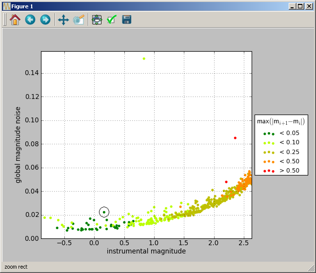
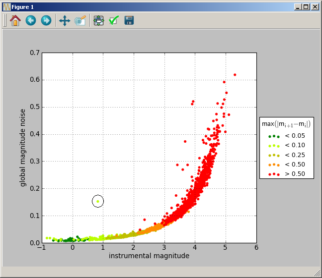
A quality flag has been given to each measured lightcurves. The best quality corresponds to “0”, and is obtained if the strongest magnitude “jump” between two consecutive values is smaller than 0.05. The mathematical condition is:

All these objects are shown in dark green on the figure. Other quality flags (and colors) are associated to the objects with stronger magnitude “jumps”.

Searching variable stars

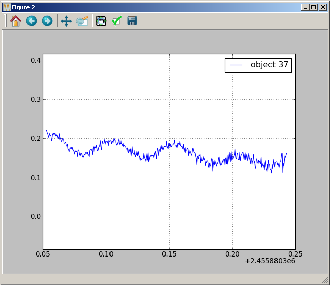
To visualise the lightcurve corresponding to a particular measured objects, do a simple right click on its point on the plot showing statistical information. Then a second figure appears, with the lightcurve.

If one right-click on the isolated green point, that is above all the other stars, then one sees the corresponding lightcurve. This is a variable star, which has been identified to be V1004 Cas.

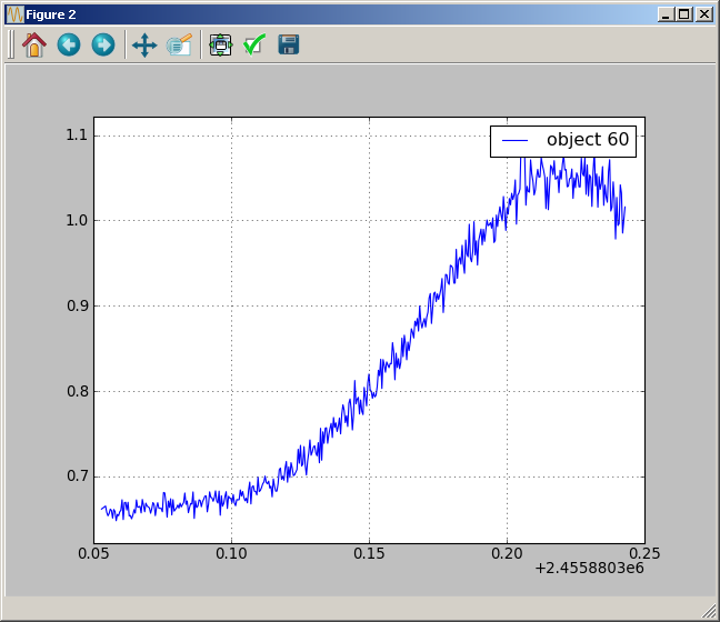
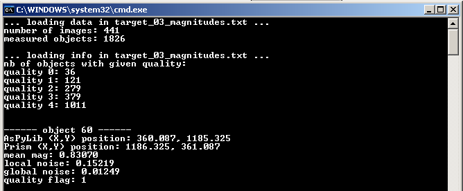
At the same moment, some information on the selected object is printed in the console window. In particular, the (X,Y) coordinates of this star on the first image are given. They allow to find out where this star actually is. Remember that in AsPyLib, the X coordinate is vertical and the first pixel is 0. This is a consequence of Python conventions. To be sure not to confuse the users, we also provide the (X,Y) coordinates valid for popular softwares as Prism, Au-dela, etc, for which X is horizontal and the first pixel is 1.

In general, only the most obvious variable stars can be identified at first sight. When zooming one can find other variable stars, with much fainter variations. For instance the dark green dot below corresponds to an unknown variable star, which has been called “JC4” by Raoul Behrend (see here).