6.4 Fitting a periodic lightcurve

Reference script

The least-square fit can be made with the following script. A similar script is provided in the file “06_cdr\Lightcurve_fitperiod.py”.

from aspylib import cdr, astro
import numpy as np
import matplotlib.pyplot as plt

#------ input files --------------------------------
Folder = u"C:\\Mesures\\"
Filelist = ["JC4_01Sept2011.txt", "JC4_14Nov2011.txt", "JC4_15Nov2011.txt"]
Filelist = [Folder + x for x in Filelist]

#------ loading data -------------------------------
alldata = cdr.load_magdata(Filelist)

#------ time correction ----------------------------
alpha = astro.hours_to_decdegrees('00:08:29.67')
delta = astro.degrees_to_decdegrees('+64:19:46.9')
alldata = cdr.time_correction(alldata, 2, [alpha,delta])

#------ performing the fit -------------------------
T0 = 2455800
period = 0.04982                #initial guess for the period, in days

popt, pcov, period, dperiod, amplitude, maxdate, mindate = cdr.fit_CDR(alldata, period, T0, nb_harmo = 2, show_results = True, show_plot = True)
plt.ylim([-0.061,0.061])
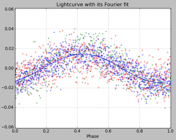
plt.title('Lightcurve with its Fourier fit')
plt.show()

Results for star JC4

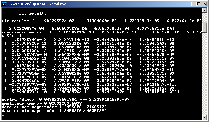
For the variable star JC4 we find the following results. With the parameter “period” set to 0.04982 we deliberately forced the fit to find the same period as CourbRot.

On the CdR-CdL website we find:

As we see we recover very similar results in both cases:

• period = 0.0498230 days (AsPyLib) / 0.0498228 days (CdR-CdL)
• period uncertainty = +/- 0.0000002 (AsPyLib) / +/- 0.0000004 days (CdR-CdL) which probably indicates the use of different noise estimates
• amplitude = 0.0289 (AsPyLib) / 0.0291 (CdR-CdL)
• heliocentric date of min magnitude = 01.9463 September 2011 in both cases.

We can note the very small value of period uncertainty, which comes directly from the very narrow width of the oscillation feature in which the fitting algorithm finally ends (see the analysis perfored here). Since it’s not clear if the minimum found by the algorithm is the right one, this uncertainty value is not yet representative.

Calculating a phase ephemeris

It is easy to calculate a phase ephemeris. This can be done by adding the following code to the script above:

#------ phase ephemeris ----------------------------
JJ = np.linspace(2455822.5, 2455842.5, 201)
print
print "------ phase ephemerids ------"
phase = (JJ-T0)/popt[0]-np.floor((JJ-T0)/popt[0])

for i,dd in enumerate(JJ):
        print dd, phase[i]

raw_input("Press Enter")