6.3 Finding the lightcurve period

Difficulty

In this section we show some of the difficulties associated with the determination of the period of a fast variable star. As we will see with an example, finding the period of a lightcurve cannot be made with a single least square fit. The reason is that the residual error of the fit strongly oscillates when you change the period, and then it’s very difficult to find out where the minimum residual is. This is well illustrated by this figure on the webpage of the CourbRot software.

All the calculations presented below correspond to the variable star JC4, discovered in September 2011 and now in the CdR-CdL database (see here).

Reference script

The following script can be used to make a fit with a fixed value of the period. Then it’s possible to look for the minimum of the residual as the period changes.

The script is based on the function cdr.fit_givenperiod(). A similar script is provided in the file “06_cdr\Lightcurve_searchperiod.py”.

from aspylib import cdr, astro
import numpy as np
import matplotlib.pyplot as plt

#------ input files --------------------------------
Folder = u"C:\\Mesures\\"
Filelist = ["JC4_01Sept2011.txt", "JC4_14Nov2011.txt", "JC4_15Nov2011.txt"]
Filelist = [Folder + x for x in Filelist]

#------ loading data -------------------------------
alldata = cdr.load_magdata(Filelist)

#------ time correction ----------------------------
alpha = astro.hours_to_decdegrees('00:08:29.67')
delta = astro.degrees_to_decdegrees('+64:19:46.9')
alldata = cdr.time_correction(alldata, 2, [alpha,delta])

#------ fit residual error -------------------------
T0 = 2455800
periods = np.linspace(0.02, 0.14, 1000)         #possible periods, in days

error = []
for period in list(periods):
        error.append(cdr.fit_givenperiod(alldata, period, T0, nb_harmo = 2))

plt.figure()
plt.plot(periods, np.sqrt(error))
plt.grid()
plt.xlabel("Period in days")
plt.ylabel("Fit error")
plt.title("Search for rotation period")
plt.show()

Measured lightcurves for star JC4

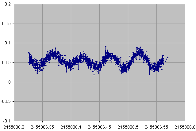
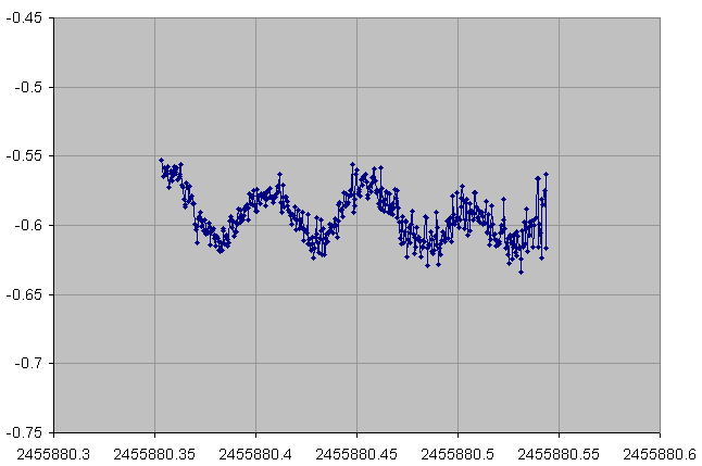
The variable star JC4 has been observed on 3 nights. The measured lightcurves are shown below in chronological order.

01 September 2011

14 November 2011

15 November 2011

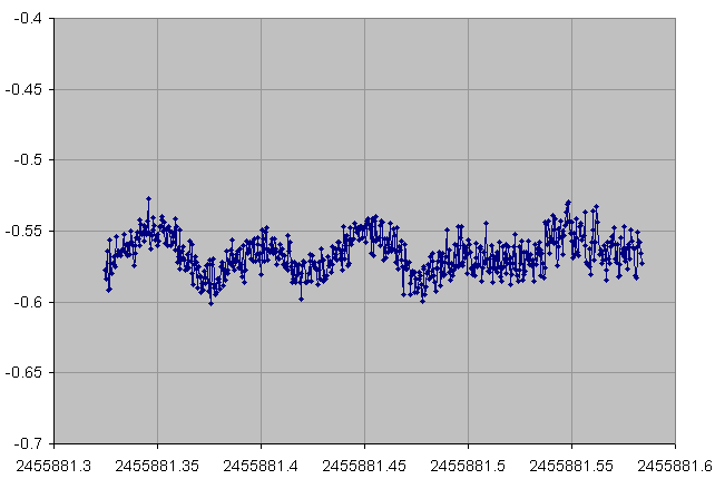
From the fast variability, weak amplitude and the regular shape (sinusoidal) of the lightcurves, JC4 has been identified to be a Delta Scuti Cepheid. This information is important because from the type of variability we can deduce the number of minima in the lightcurve. In most cases:

• a pulsating star will have a single minimum per cycle
• an eclipsing star will have two minima per cycle

Possible periods for star JC4

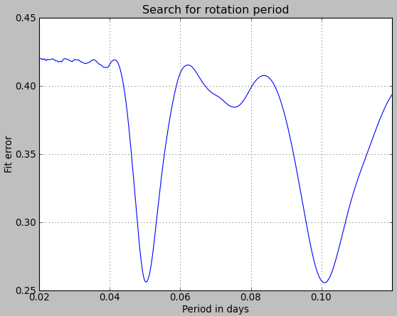
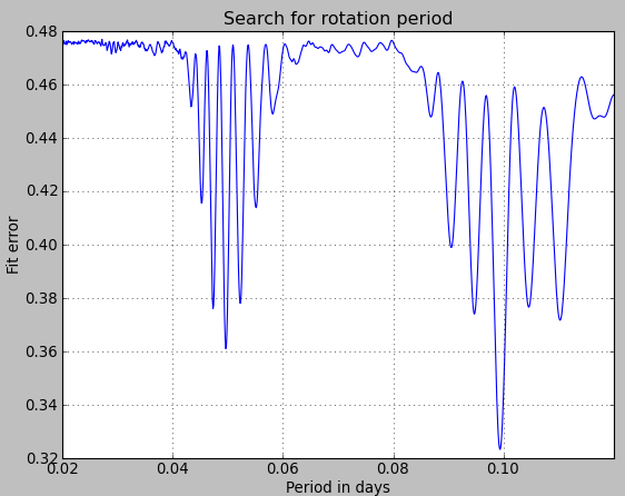
If we keep only the first observation of JC4 (01 September) then we get the following curve of the fit residual as a function of period. On this curve, we see two minima around 0.05 days and 0.10 days. Using our assumption of a Delta Scuti star, we will keep the value of 0.05 days for the period.

Now if we take the two last observations (14 and 15 November) we find the following curve. The use of two consecutive nights creates “oscillations”. The strongest residual minimum relevant for JC4 is found around 0.0497 days.

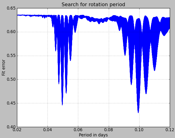
When we take all three observations, the oscillations become so fast that it is difficult to resolve them. A highly resolved calculation was done in about two hours. We got the following figure.

Zooming in around the value 0.05 we get:

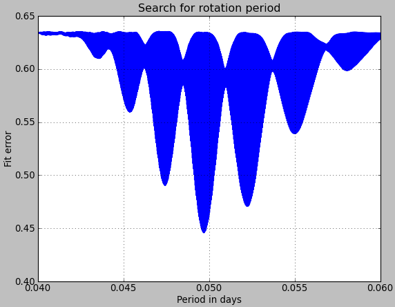
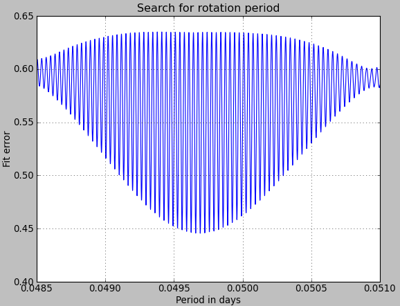
Here comes the problem. From this figure, we see several extremely close minima of the fit residual, obtained for slightly different period values. If we zoom in further we can find the absolute minimum.

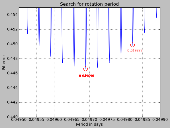
From our calculation, the best period seems to occur at 0.049690 days. We are using a standard least-square algorithm where the measurements are weighted according to the noise values.

With CourbRot, the solution at 0.049823 days was the optimum. This comes probably from the fact that slightly different noise values have been used in both softwares. It is also possible that a few erroneous measurement points have been removed by the CourbRot algorithm.

This example illustrates well how difficult the identification of the period is. In the end, both solutions (0.049690 and 0.049823 days) are equally plausible. For JC4, some more observations may be needed to confirm the final period value.