3.4 Geometrical transformations

Simple script

The following script can be used to

• load an existing image,
• display it,
• apply some geometrical transformation on it,
• display the transformed imaged,
• and then save the transformed image under a different name

# -*- coding: iso_8859_1 -*-
from aspylib import astro

#------ image names ------
Folder = u"C:\\Images\\"
Image_in = [Folder + "Image-in.fit"]
Image_out = [Folder + "Image-out.fit"]

#--- loads image data and headers ---
data = astro.get_imagedata(Image_in)
headers = astro.get_headers(Image_in)

#--- display image, apply transformation, display transformed image ---
astro.display(data, title='initial image')
# here geometrical transformation (see examples below)
# the result is data2
astro.display(data2, title='transformed image')

#--- saves modified image ---
astro.save_imagelist(data2, headers, Image_out)

raw_input()

Available transformations

At the moment the following transformations can be used. Simple transformations:

• vertical mirror
• horizontal mirror
• rotation 90 deg
• rotation 180 deg
• rotation 270 deg

Transformations with interpolation required:

• translations (with non-integer shifts)
• rotations (the rotation axis can be anywhere inside, or outside the image)
• scaling (zoom in, zoom out, with non-integer scaling factors)

All the transformations can be applied equivalently on single images or lists of images.

Mirror symmetries, 90 deg rotation

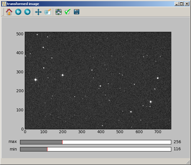
The vertical mirror is implemented with:

data2 = astro.mirror_vert(data)

The obtained image is:

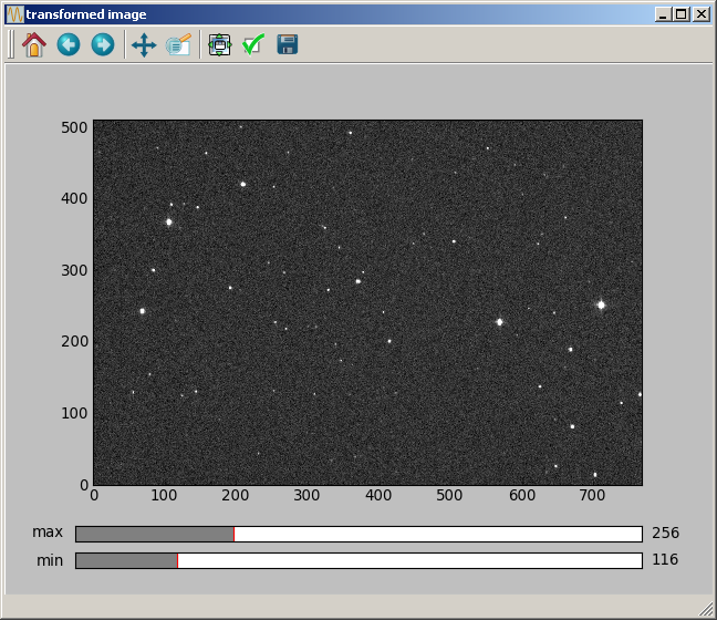
The horizontal mirror is implemented with:

data2 = astro.mirror_horiz(data)

The obtained image is:

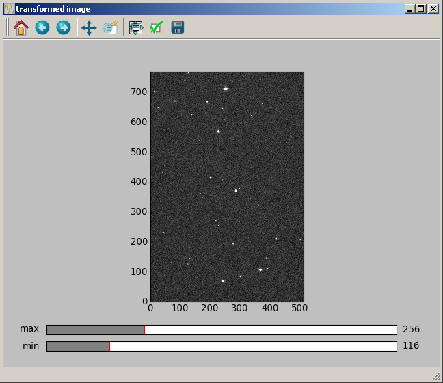
A 90 deg rotation is implemented with:

data2 = astro.rot_90(data)

The obtained image is:

Rotations by 180 or 270 deg are implemented with similar instructions (rot_180 and rot_270).

Pixel interpolation

The translations, rotations and scalings can be calculated with bilinear or B-spline interpolation (with order 2,3,4,5,6,7,8 or 9). The B-spline interpolation is implemented with an algorithm programmed by P.Thevenaz, available here. Many thanks to him for this very nice piece of code, all the documentation and his detailed responses to some questions I asked.

For astronomy, one key aspect is that both the bilinear and Bspline interpolations algorithm will not affect the normalisation of the image, for an isometric transformation (a transformation that keeps distances unchanged: translation and rotation, but not scaling). Thus the bilinear and Bspline algorithm can, in principle, be used for photometry.

The other aspect is the accuracy of the interpolation algorithm. The bilinear interpolation has not a very good reputation, because for non-integer shift values, a translation will smooth the background noise of the image, completely changing its aspect. The Bspline algorithm is much better and does not create such image degradation.

The accuracy of the interpolation algorithms has been quantified in the section VIII of this paper, where about 40 different interpolation algorithms are compared. Three different pictures are considered, and are rotated 15 times by 24 degrees. The obtained image, after the 15 consecutive rotations, is compared to the original image. If the transformation is ideal, then the initial image should be recovered (since 24*15 deg = 360 deg). From the comparison it is clear that the Bspline algorithm is one of the best approaches known. In fact, the Bspline interpolation with order 3 is a standard algorithm in image processing.

Bspline interpolation with order 3 (also called “cubic Bspline”) is the interpolation that we recommend to use.

Translations

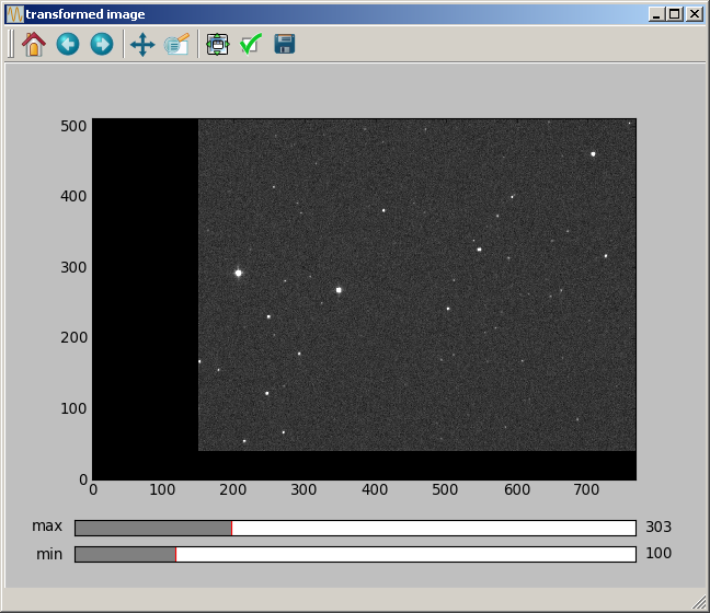
A translation of 40.3 pixels in the vertical direction, 150.2 pixels in the horizontal direction can be made with:

data2 = astro.translate_Bspline(data, [40.3, 150.2], 3)

The first argument is the input image data, the second argument is a two elements list giving the shift [vertical shift, horizontal shift], and the last argument is the order of the Bspline transformation. The obtained image is the following:

For information, the equivalent function with bilinear interpolation is:

data2 = astro.translate_bilinear(data, [40.3, 150.2])

Rotations

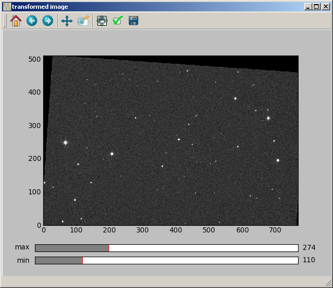
For the rotation, an angle must be specified, and the (vertical, horizontal) position of the rotation axis. A rotation of 4 deg with the axis at coordinates (100.2, 20.4) is made with:

data2 = astro.rotate_Bspline(data, [100.2, 20.4], 4.0, 3)

The obtained image is:

Scaling

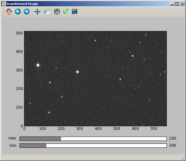
For the scaling, in addition to the scaling factor, the (vertical, horizontal) position of a pixel that will not be moved must be provided. Non-integer values can be specified for this position. A scaling of a factor of 1.5 with the unchanged pixel being at (100.2, 20.4) is made with:

data2 = astro.scaling_Bspline(data, [100.2, 20.4], 1.5, 3)

The obtained image is:

Effect of computer screen with rectangular pixels

On some computer screens, it can happen that a rotated image seems not to have square corners any more. This effect is not linked to the image rotation which was computed correctly. It comes from the screen which has rectangular pixels !

EXACTLY THE SAME EFFECT is observed with most image processing softwares for astronomy (IRIS, AUDELA, PRISM, ...). When displaying an image, AsPyLib is doing the same as these classical softwares:

• it does not detect the pixel physical size, which can be rectangular on some screens
• when displaying an image, it only makes sure that the scale (= number of image pixels per screen pixel) is the same on both vertical and horizontal directions.

If an image calculated and displayed with AsPyLib is found to have a corner larger than 90 deg, it can be saved and displayed with one of these software. Then the corner will still be larger than 90 deg. But, after applying a diagonal mirror to it:

• in PRISM: Transformation –> Quart de Tour
• in Audela: PreProcessing –> Diagonal Mirror
• in IRIS: Geometrie –> Permutation –> Diagonale

The transformed image will have a corner now smaller than 90 deg !