3.6 Fitting stars

Simple script for stars fitting

Once the coordinates of a star are known, a small part of the image around the star can be defined, and used to perform a PSF fitting on the star. In AsPyLib, the following PSF models are available:

• circular gaussian
• elliptical gaussian
• circular moffat
• elliptical moffat

Here is a simple script that can be used to fit stars on an image with a 2D circular gaussian

# -*- coding: iso_8859_1 -*-
from aspylib import astro

#--- loads image data ---
Image = ["C:\\Images\\Image-1.fit"]
data = astro.get_imagedata(Image)

#--- display image ---
fig, ax = astro.display(data)
while 1:
    print
    xy = astro.select(fig, ax, 1)
    x,y = xy[0]
    param = astro.fit_gauss_circular([x-10,y-10],data[x-10:x+11, y-10:y+11])
    print "floor (in ADU)   =", param[1]
    print "height (in ADU)  =", param[2]
    print "x0 (in pixels)   =", param[3]
    print "y0 (in pixels)   =", param[4]
    print "fwhm (in pixels) =", param[5]

raw_input()

After right-clicking on two objects, the text displayed in the console looks like:

--- loading FITS image ---
Image-1.fit

x= 251 y= 55
floor (in ADU) = 193.484201821
height (in ADU) = 19014.3851849
x0 (in pixels) = 251.888470768
y0 (in pixels) = 55.9261718203
fwhm (in pixels) = 2.06287051386

x= 369 y= 661
floor (in ADU) = 163.311263174
height (in ADU) = 6601.31089411
x0 (in pixels) = 367.875223306
y0 (in pixels) = 660.94550699
fwhm (in pixels) = 2.1845135079

Circular gaussian PSF

The traditional equation for a circular gaussian PSF is:

To fit a star with a circular gaussian, AsPyLib is using a slightly different form of this equation:

The fit is performed by optimising 5 parameters: S0, S1, x0, y0, w. This equation has been chosen because it involves less calculation than the other one. This helps to reduce the execution time. It is also important to take the absolute value of w to avoid positive exponentials.

The following instruction is used to make the fit:

results = astro.fit_gauss_circular([x-10,y-10],data[x-10:x+11, y-10:y+11])

When the calculation is finished, astro.fit_gauss_circular() returns 6 parameters:

• results[0] is just the maximum pixel value in the selected subimage, not a fit parameter but a useful information.
• results[1] = S0 is the level of the sky background
• results[2] = S1 is the amplitude of the gaussian PSF
• results[3] = x0 and results[4] = y0 give the star position along x and y directions.
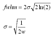
• results[5] = fwhm is the PSF full width half maximum and is calculated from w with the equations below

Elliptical gaussian PSF

The equation for the elliptical gaussian is traditionally defined with matrices:

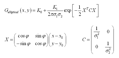
This equation is equivalent to:

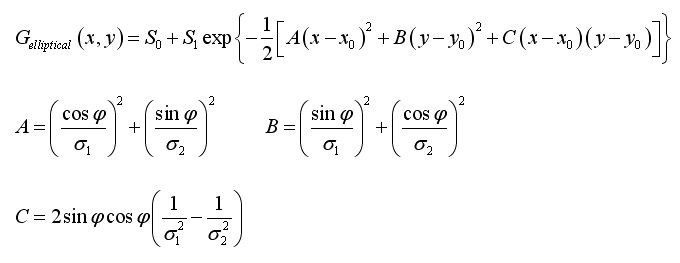
The fit is performed by AsPyLib by optimising 7 parameters: S0, S1, x0, y0, sigma1, sigma2, phi. The following instruction is used:

results = astro.fit_gauss_elliptical([x-10,y-10],data[x-10:x+11, y-10:y+11])

When the calculation is finished, astro.fit_gauss_elliptical() returns 8 parameters:

• results[0] is just the maximum pixel value in the selected subimage, not a fit parameter but a useful information.
• results[1] = S0 is the level of the sky background
• results[2] = S1 is the amplitude of the gaussian PSF
• results[3] = x0 and results[4] = y0 give the star position along x and y directions
• results[5] and results[6] give the smallest and largest star full width half maximum (FWHM) sizes. The FWHMs are calculated from sigma1 and sigma2 with the same equation as for the circular gaussian
• results[7] = phi is the angle, in degrees, that gives the direction of the largest FWHM, measured starting from x (vertical direction) in the clockwise direction. This angle is between -90 deg and +90 deg.

Circular moffat PSF

For the circular moffat PSF, AsPyLib is using this equation:

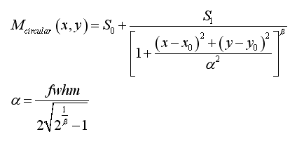
The fit is performed by AsPyLib by optimising 6 parameters: S0, S1, x0, y0, fwhm, beta. The following instruction is used:

results = astro.fit_moffat_circular([x-10,y-10],data[x-10:x+11, y-10:y+11])

When the calculation is finished, astro.fit_moffat_circular() returns 7 parameters:

• results[0] is just the maximum pixel value in the selected subimage, not a fit parameter but a useful information.
• results[1] = S0 is the level of the sky background
• results[2] = S1 is the amplitude of the moffat PSF
• results[3] = x0 and results[4] = y0 give the star position along x and y directions
• results[5] = fwhm is the PSF full width half maximum
• results[6] = beta.

Elliptical moffat PSF

For the elliptical moffat PSF, AsPyLib is using this equation:

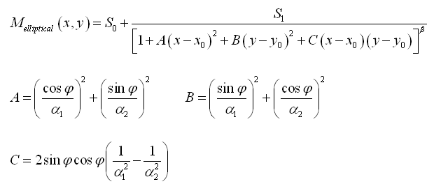
The fit is performed by AsPyLib by optimising 6 parameters: S0, S1, x0, y0, fwhm1, fwhm2, phi, beta. The parameters fwhm1 and fwhm2 are calculated from alpha1, alpha2 and beta with the same equation as for the circular moffat. To perform the fit the following instruction is used:

results = astro.fit_moffat_elliptical([x-10,y-10],data[x-10:x+11, y-10:y+11])

When the calculation is finished, astro.fit_moffat_elliptical() returns 9 parameters:

• results[0] is just the maximum pixel value in the selected subimage, not a fit parameter but a useful information.
• results[1] = S0 is the level of the sky background
• results[2] = S1 is the amplitude of the moffat PSF
• results[3] = x0 and results[4] = y0 give the star position along x and y directions
• results[5] and results[6] give respectively the smallest and largest star full width half maximum (FWHM) sizes
• results[7] = phi is the angle, in degrees, that gives the direction of the largest FWHM, measured starting from x (vertical direction) in the clockwise direction. This angle is between -90 deg and +90 deg.
• results[8] = beta.